Search
Steps
- Formulate goal
- Formulate problem
- Find solution
Types of Search
| Type | Examples |
|---|---|
| Single-Agent | Traveling Salesperson 8-Puzzle (Sudoku) Wiring of VLSI circuits Finding faults in vehicle |
| Two-Agent | Chess Tic-Tac-Toe Checkers Go Tzaar |
| Constraint-Satisfication | Scheduling 8-Queens F-Block |
Parts of Search
Agents
| Type of Agents | |
|---|---|
| Intelligent/ Problem Solving/ Rational Agents | has goals and tries to perform a series of actions that yield the best outcome/achieve a goal |
| Reflex Agents | Don’t think about consequences of its actions, and selects an action based on current state of the world. |
Keywords
| Keyword | Meaning | |
|---|---|---|
| State | Description of possible state of the world Includes all features relevant to problem | |
| Initial/ Start State | State from where agent begins the search | |
| Goal State | State where success is attained, which we want to reach Multiple goal states can exist | |
| Goal Test | Function that observes current state and returns whether goal state is achieved/not | |
| Action | Function that maps transitions from one state to another | |
| Problem | Definition of general problem as search problem | |
| Solution | Sequence of actions that help go from initial state to goal state | |
| Solution cost | Cost associated to perform solution | |
| Search | Process of looking for solution | |
| State Space | Set of all states that are possible and can be reached in an environment/system. |  |
| State space size | Total number of states. Counted using fundamental counting principle. | |
| Search Tree | Tree representation of search problem. | 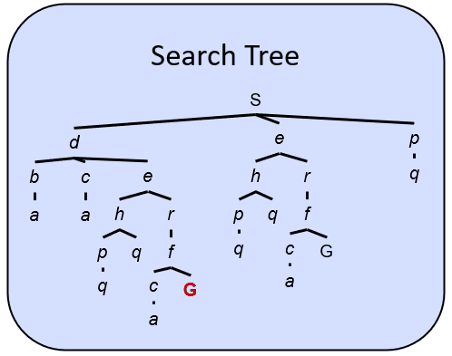 |
Search Type
IDK
| Type | Path is relevant? | Direction | ||
|---|---|---|---|---|
| Planning | Sequence of actions | ✅ | Backward chaining |  |
| Diagonosis | ✅ | Forward chaining |  | |
| Identification | Assignment to variables | ❌ |
Information
| Information | Other names | Comment |
|---|---|---|
| Uninformed | Blind Brute-Force Undirected | |
| Informed | Tends to be faster |
Search Property
| Property | Meaning |
|---|---|
| Completeness | Algo guaranteed to find soln in a finite duration \(\iff \exists\) a soln |
| Optimality | Algo guaranteed to find least cost path to goal state |
Heuristic
A heuristic function \(h(x)\) is an estimated cost from one node to another
- Heuristics are problem-specific
- Over-estimating heuristic is better than under-estimating
- As heuristics get closer to the true cost, you will expand fewer nodes but usually do more work per node to compute the heuristic itself
Eg: Manhattan distance, Euclidean distance
Characteristics
Consider
- \(h(a, b)\) is heuristic from \(a\) to \(b\)
- \(c(a, b)\) is true cost from \(a\) to \(b\)
| Characteristic | Definition | Comment | Implication |
|---|---|---|---|
| Admissible | \(h(x, G) \le c(x, G) \quad \forall x\) | Heuristic never overestimates true cost | Admissible slows down bad plans, but never outweigh true costs Inadmissible/pessimistic compromises optimality but with lower (better) search time |
| Consistent | \(\vert h(x_1, G) - h(x_2, G) \vert \le c(x_1, x_2)\) where \(x_2\) is an intermediate node b/w \(x_1\) and \(G\) | Every consistent heuristic is also admissible | \(f\) value along path never decreases You can skip checking for shortest path when a node is encountered 2nd time. |
| Informedness/ Domination | \(h_1(x, G) \ge h_2(x, G) \quad \forall x\) where \(h_1, h_2\) are admissible | \(h_1\) is more informed than \(h_2\) \(h_1\) dominates \(h_2\) | |
| Semi-lattice of heuristics | \(\max(h_1, h_2)\) is admissible | ||
| Trivial heuristic | Bottom of lattice is zero heuristic \(\implies\) top of lattice is exact heuristic |

Search Algorithms
| Search Type | Algo | Comment | Complete | Optimal | Time Complexity | Space Complexity | Disadvantage | Advantage | Hyperparameter | |
|---|---|---|---|---|---|---|---|---|---|---|
| Uninformed | DFS | Keep picking left-most node possible | Explore deepest node from start node (Stack - LIFO) | ❌ ✅ (if no cycles) | ❌ | \(O(b^m)\) | \(O(bm)\) | May get “lost” deep in graph, missing the shortest path | Avoids searching “shallow states” for long solution | |
| BFS | Traverse left to right, level by level | Explore shallowest node from start node (Queue - FIFO) | ✅ | ✅ | \(O(b^{m_s} + 1)\) | \(O(b^{m_s}+1)\) | High memory usage if states have high avg no of children | Always finds shortest path | ||
| Iterative-Deepening | Combination of DFS and BFS) | Perform DFS for every level DFS with depth bound | Not necessarily | \(O(b^d)\) | \(O(bd)\) | Repeated work (negligible though: \(O(1/b)\)) | Prevents DFS from getting lost in infinite path | Depth threshold | ||
| UCS (Uniform Cost)/ Branch & Bound | Orders by path/backward cost \(c(i, x)\) | Explore least cost node from start node | ✅ (\(\iff\) all costs are non-negative) | ✅ | \(O(b^m)\) | \(O(b^m)\) | Explores options in “every direction” | Keeps cost low | ||
| Bi-Directional | Performed on search graph | Two simultaneous search - forward search from start vertex toward goal vertex and backward search from goal vertex toward start vertex | ✅ | ✅ \(\iff\) we use BFS in both searches | \(O(b^{d/2})\) | \(O(b^{d/2})\) | Can prune many options | - Which goal state(s) to use - Handling search overlap - Which search to use in each direction - 2 BFS searches | ||
| Informed | Greedy/Best-First | Explore the node with lowest heuristic value which takes closer to goal Orders by goal proximity/forward cost \(h(x, G)\) | Similar to UCS, but with a priority queue | ❌ | ❌ | \(O(b^m)\) | \(O(b^m)\) | Tentative May directly go to wrong end state May behave like a poorly-guided DFS | Helps find solution quickly | |
| A* | Explore the node with lowest total cost value \(f = C(i, x) + h(x, G)\) | Uses priority queue Combination of UCS & Greedy | ✅ | ✅ (\(\iff\) heuristic is admissible) | \(O(b^m)\) | \(O(b^m)\) | ||||
| Hill-Climbing | Basically gradient-descent | ❌ | ❌ | \(O(bm)\) | \(O(b)\) | Irreversible If bad heuristic, may prune away goals Stuck at local minima/maxima Skips ridges Plateaus | Fast Low memory | |||
| Beam | Compromise b/w hill-climbing & greedy | \(n=1:\) Hill-Climbing \(n=\infty:\) Best-First \(n \in (1, \infty) :\) Beam width (no of children to search) | ❌ | ❌ | \(O(nm)\) | \(O(bn)\) | ||||
| IDA* (Iterative Deepening A *) | Similar to Iterative Deepening, but uses A* cost threshold | Increase always includes at least one new node | ✅ | ✅ | \(O(b^m)\) | \(O(m)\) | Some redundant search, but negligible Dangerous if continuous \(h\) values or if \(h\) values very close to threshold | Ensures search never looks beyond optimal cost soln | - Threshold - \(h\)(root) - \(f\)(min_child) min_child is the cut off child with min \(f\) | |
| RBFS (Recursive Best-First/Greedy) | Linear space variant of \(A^*\) | Backtrack if current node is worse than next best alternative Perform \(A^*\) but discard subtrees when performing recursion Keep track of alternative (next best) subtree Expand subtree until \(f>\) bound Update \(f\) before (from parent) and after (from child) recursive call | \(O(2^m)\) | \(O(bm)\) | Stores more info than IDA* | More efficient than IDA* | ||||
| SMA* | Simplified Memory-Bounded A* | Perform A*, but when memory is full, discard worst leaf (highest \(f\)) Back value of discarded node to parent | ||||||||
| Hill-Climbing | Random restart helps overcome local maxima/minima Random sideways moves help escape from - shoulders - loop on flat maxima | ❌ Trivially complete with random restart | ❌ | Irreversible steps Skips ridges | Fast Low memory requirement | |||||
| Local Beam | \(k\) hill climbs | Choose \(k\) random successors Similar to natural selection | ❌ | ❌ | Inefficient All \(k\) states end up on same local hill | \(k\) | ||||
| Simulated Annealing | Trade-off b/w hill-climbing & random search | Randomness at high “temperature” When temperature cools, reduce prob of random moves | Can find global optima when temperature chosen correctly | Temperature | ||||||
| Genetic Algorithm |
where
- \(b =\) max branching factor (nodes at each level)
- \(m=\) depth
- \(m_s =\) depth of shallowest solution
- \(C^*\) is optimal path cost
- \(\epsilon\) is minimal cost between 2 nodes
Fringe is a priority queue
Iterative Improvement Search
Local search
Hill-climbing, local beam, simulated annealing, genetic
Appropriate when only reaching goal state is required; solution path is irrelevant
IDK

Graph Search
Helps avoid repeated states - Do not return to parent/grand-parent states - Do not create solution paths with cycles - Do not generate repeated states as options (need to store & check more states)
Implementation
- Data structures
- Tree (as usual)
- Set of expanded (visited/closed) nodes
- Traversal
- Visit node from open set
- Check if visited previously
- If visited, skip node and go to step 1
- Else
- expand node
- add node to closed set
- add children to open set
Implications
- Completeness maintained
- Optimality is not guaranteed