Computer Vision
Extraction, analysis and comprehension of useful information from image(s)
Used for Navigation & Mapping
An image may be defined as a 2D function \(f(x, y)\) where
- \(x, y\) are spatial coordinates
- value of \(f\) gives the intensity at a point
Channels
- For a gray-range image, intensity is given by just one ‘channel’
- For color images, intensity is given by 3d vector (3 channels): RGB
Conversion from analog to a “digital image” requires both coordinates and intensity to be digitized
- Sampling: Digitizing the coordinates
- Quantization: Digitizing the intensity
Types of images
| Binary Image | Intensity Image | Color Image | |
|---|---|---|---|
| Black and white | Data matrix whose values have been scaled to represent intensities | Intensity image with 3 channels (RGB) | |
| Values | 0/1 | Usually scaled to [0, 255] or [0, 1] |
Image Quantization
Transforming a real valued sampled image into one with a finite number of distinct values
Eg: rounding the digits, setting a max/min range
Convolution Filters
- Low-pass: noise removal, blur
- High-pass: edge detection, sharpening
Averaging
Gaussian
Nearest neighboring pixels have the most influence
Center of the filter matrix will be larger than the edges and the corners
Variance of the filter determines the smoothing
Median
Salt and pepper noise reduction
Bilateral
Blur while maintaining sharp edges
Slower
Edge Detection
Look for a neighborhood with strong signs of change
- Surface normal discontinuity
- Surface color discontinuity
- Illumination discontinuity
- Depth discontinuity
Kernel
- Kernel should be symmetric
- Normalization required to make the sum of elements in the filter as 1
Derivative will be non-zero at edges
Discrete gradient
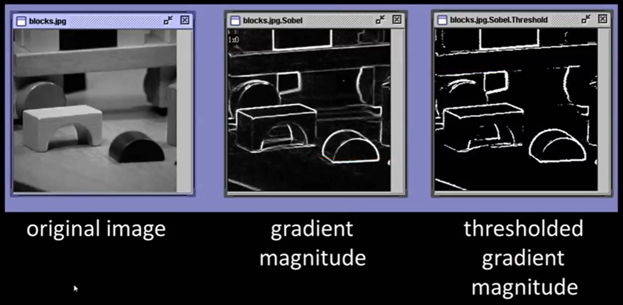
Sobel Operator
- Sobel
- Prewitt
- Roberts
Difficulties
- Neighborhood size
- Change detection
Canny Edge Detection
Robust and flexible
- Noise reduction
- Calculating intensity gradient
- Suppression of false edges
- Hysteresis thresholding
Thresholding: \(\vert \vert \nabla f \vert \vert\) are compared with 2 threshold values
- If \(\vert \vert \nabla f \vert \vert > T_h\), those pixels are associated with solid edges and included in the final edge map
- If \(\vert \vert \nabla f \vert \vert < T_l\), those pixels are suppressed and excluded from final edge map
- All other pixels are marked as “weak” edges, and become candidates for final edge map
- If weak pixels are connected to solid pixels, they are also included in final edge map
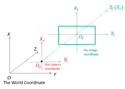
Camera Calibration
Estimates parameters of lens and image sensor, to be used for
- Correction of lens distortion
- Object measurement
- Determine location of camera in scene
- Estimate depth using stereo camera
- Estimate 3D structure from camera motion
Camera
Converts 3D world into 2D image $$ \begin{aligned} x &= PX \ \begin{bmatrix} X \ Y \ Z \end{bmatrix} &= \begin{bmatrix} p_1 & p_2 & p_3 & p_4 \ p_5 & p_6 & p_7 & p_8 \ p_9 & p_{10} & p_{11} & p_{12} \end{bmatrix} \begin{bmatrix} X \ Y \ Z \ 1 \end{bmatrix} \end{aligned} $$ where
- \(x =\) homogeneous image
- \(P =\) camera matrix
- \(X =\) homogeneous world point
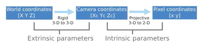
Parameters
| Intrinsic/Internal | Extrinsic/External | |
|---|---|---|
| Allows mapping between pixel coordinates and camera coordinates in the image frame | Describe orientation and location of camera | |
| Example | Optical center Focal length Radial distortion of coefficients of lens | Rotation of camera Translation of camera wrt world coordinate system |
Pinhole Camera Model
Basic camera model without a lens. Light passes through aperture and projects an inverted image on the opposite side of the camera.
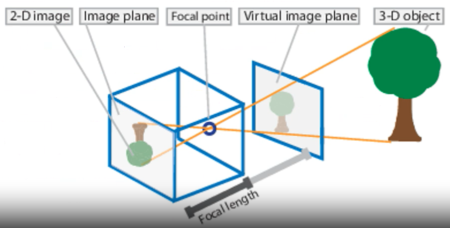
Visualize the virtual image plane in front of the camera and assume that it is containing the upright image of the scene $$ \begin{aligned} w \begin{bmatrix} x & y & 1 \end{bmatrix} &= \begin{bmatrix} X & Y & Z & 1 \end{bmatrix} P \ P &= \begin{bmatrix} R \ T \end{bmatrix} k \ k &= \begin{bmatrix} f_x & s & c_x \ 0 & f_y & c_y \ 0 & 0 & 1 \end{bmatrix} \end{aligned} $$ where
- \(w=\) scale factor
- \(P=\) camera matrix represents the camera specifications
- \(R=\) Rotation
- \(T=\) Translation
- \(k=\) Intrinsic matrix
- \(F =\) focal length in world units, usually in mm
- \((p_x, p_y) =\) size of pixel in world units
- \(f_x, f_y = \dfrac{F}{p_x}, \dfrac{F}{p_y} =\) focal length in pixels
- \(\begin{bmatrix}c_x & c_y \end{bmatrix}=\) optical center (principal point) in pixels
- \(s = f_x \tan \alpha\) skew coefficient
- non-zero if image axes are not perpendicular
- 1 pixel \(\approx 1/96 \text{inch}\)
Distortion
| Barrel (Radial) | Pincushion (Radial) | Tangential/Decentering | |
|---|---|---|---|
| Meaning | Straight lines of actual world appear curved outward | Straight lines of actual world appear curved inward | Image appears to slanted & stretched |
| -ve radial displacement | +ve radial displacement | ||
| Cause | Unequal light bending (rays bent more at lens’ border than at center) Before hitting the image sensor, the light ray is shifted radial inward/outward from its optimal point | Unequal light bending (rays bent more at lens’ border than at center) Before hitting the image sensor, the light ray is shifted radial inward/outward from its optimal point | Picture screen/sensor is at an angle wrt lens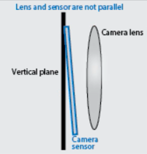 |
| Example | 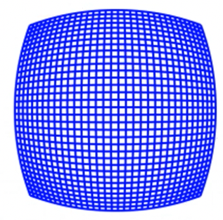 | 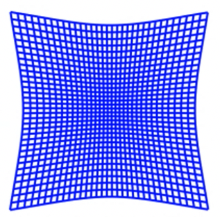 | 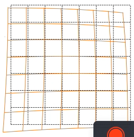 |
Radial distortion coefficients model
where
- \(x_\text{distorted}, y_\text{distorted}\) are distorted points
- \(x, y\) are undistorted and dimensionless pixel location in normalized image coordinates format, calculated from pixel coordinates by translating to optical center and dividing by focal length in pixels
- \(k_1, k_2, k_3\) are radial distortion coefficients of the lens
- \(r^2 = x^2 + y^2\)
Tangential distortion coefficients model
Distortion Removal
- Calibrate camera and obtain intrinsic camera parameters
- Control percentage of undersized pixels in undistorted image by fine-tuning camera matrix
- Use revised camera matrix to remove distortion from image