03 Data Preprocessing
Preprocessing Techniques
You don’t have to apply all these; it depends. You have to first understand the dataset.
| Technique | Meaning | Advantage | Disadvantage |
|---|---|---|---|
| Aggregation | Combining/Merge data objects/attributes Continuous: Sum, mean, max, max, min, etc Discrete: Mode, Summarization, Ignoring | - Low processing cost, space, time - Higher view - More stable | Losing details |
| Sampling | Creating representative subset of a dataset, whose characteristics are similar to the original dataset | ||
| Dimensionality Reduction | Mathematical algorithm resulting in a set of new combination of old attributes | Eliminate noise and unnecessary features Better understandability Reduce time, memory and other processing cost Easier visualization | Getting the original data is not possible after transformation |
| Feature Subset Selection | Removing irrelevant and redundant attributes | Same as ^^ | Extra resources required |
| Feature Creation | Create new attributes that can capture multiple important features more efficiently | ||
| Discretization | Convert continuous attribute into categorial/discrete (for classification) | ||
| Binarization (Encoding) | Convert continuous/categorical attribute into binary (association mining) | ||
| Attribute Transformation | Mathematical transformations |
Feature selection and Dimensionality reduction are used for biomarkers analysis
Types of Sampling
Random Sampling
| Random Sampling | Data object put back into original population? | Duplicates? |
|---|---|---|
| With replacement | ✅ | ✅ |
| Without replacement | ❌ | ❌ |
Problem
It may lead to misclassification, as not all classes are represented proportionally in the sample.
Stratified Sampling
Different types of objects/classes with different frequency are used in the sample.
Useful especially in imbalanced dataset, where all the classes have large variation in their counts.
Ensures all classes of the population are well-represented in the sample.
Steps
- Draw samples from each class
- equal samples, or
- proportional samples, using % of the total of all classes
- Gives us imbalanced dataset
- Combine these samples into a larger sample
Progressive/Adaptive Sampling
Useful when not sure about good sample size
Computationally-expensive
Steps
flowchart LR
s["Start with small sample (100-1000)"] -->
a[Apply data mining algorithm] -->
e[Evaluate results] -->|Increase Sample Size| s

e -->|Best Result Obtained| st[/Stop/]
Data Augmentation
- Images
- Flip
- Rotation
- Adding noise
- Warping
- Mixup
- Convert labels
- \(x' = \lambda x_i + (1-\lambda) x_j; y' = \lambda x_i + (1-\lambda) x_j\)
-
-
Fit it to a distribution
Dimensionality Reduction Algorithms
| Technique | Working | Reduce dimensionality while | Learning Type | Comment | No Hyperparameter Tuning Required | Fast | Deterministic | Linearity |
|---|---|---|---|---|---|---|---|---|
| LDA | Maximize distance between classes | Separating pre-known classes in the data | Supervised | ✅ | ✅ | ✅ | Linear | |
| PCA/ SVD using PCA | Maximize variance in data | Generating clusters previously not known | Unsupervised | \(2k\) contaminated points can destroy top \(k\) components | ✅ | ✅ | ✅ | Linear |
| MDS | ^^ | Unsupervised | ❌ | ❌ | ❌ | Non-Linear | ||
| t-SNE | ^^ | Unsupervised | ❌ | ❌ | ❌ | Non-Linear | ||
| UMAP | ^^ | Unsupervised | ❌ | ✅ | ❌ | Non-Linear |
Feature Selection
flowchart LR

Attributes -->
ss[Search Strategy] -->
sa[/Subset of Attributes/] -->
Evaluation -->
sc{Stopping Criterion Reached?} -->
|No| ss

sc -->
|Yes| sel[/Select Attributes/] -->
Something
Mutual Information
Mutual information (MI) between two random variables is a non-negative value, which measures the dependency between the variables. It is equal to zero if and only if two random variables are independent, and higher values mean higher dependency. The function relies on nonparametric methods based on entropy estimation from k-nearest neighbors distances.
Brute Force Approach
Consider a set with \(n\) attributes. Its power set contains \(2^n\) sets. Ignoring \(\phi\), we get \(2^{n-1}\) sets.
Steps
- Evaluate the performance of all possible combinations of subsets
- Choose the subset of attributes which gives the best results
Embedded Approach
The data mining algorithm itself performs the selection, without human intervention
Eg: A decision tree automatically chooses the best attributes at every level
Builds a model in the form of a tree
- Internal nodes = labelled with attributes
- Leaf nodes = class label
Filter Approach
Independent of data mining algorithm
flowchart LR
o[(Original<br /> Feature Set)] -->
|Select<br /> Subset| r[(Reduced<br /> Feature Set)] -->
|Mining<br /> Algorithm| Result
eg: Select attributes whose evaluation criteria(pairwise correlation/Chi2, entory) is as high/low as possible
Wrapper Approach
Use the data mining algorithm (capable of ranking importance of attributes) as a black box to find best subset of attributes
flowchart LR
o[(Original<br /> Feature Set)] -->
s[Select<br /> Subset] -->
dm[Mining<br /> Algorithm] -->
r[(Reduced<br /> Feature Set)] & s

subgraph Black Box["Ran n times"]
    s
    dm
end
Feature Engineering
Feature extraction
Mapping data to new space
- Time series data \(\to\) frequency domain
- For eg, fourier transformation
Feature construction
- Construct interaction terms from existing features
- Eg
- Area = length * breadth
- Density = mass/volume
Discretization
-
Sort the data in ascending order
-
Generate
-
\(n-1\) split points
-
\(n\) bins \(\to\) inclusive intervals (specified by the analyst)
-
Then convert using binarization. But, why?
Types
| Equal-Width Binning | Equal-Frequency Binning | |
|---|---|---|
| Analyst specifies | No of bins | Frequency of data objects in each bin |
| Width | \(\frac{\text{Max-Min}}{\text{No of bins}}\) | |
| Make sure atleast \(n-1\) bins have the correct frequency |
Binarization
| Method 1 | One-Hot Encoding | |
|---|---|---|
| For \(m\) categories, we need ___ digits | \(\lceil \log_2 m \rceil\) | \(m\) |
| No unusual relationship | ❌ | ✅ |
| Fewer variables? | ✅ | ❌ |
Attribute Transform
| \(x'\) | Property | |
|---|---|---|
| Simple | \(x^2, \log x, \vert x \vert\) | |
| Min-Max Normalization | \(\frac{x - x_{\text{min}}}{x_{\text{max}} - x_{\text{min}}}\) | \(0 \le x \le 1\) |
| Standard Normalization | \(\frac{x-\mu}{\sigma}\) | \(\mu' = 0, \sigma' = 1\) |
Naming
| Feature Transform | Input variables |
| Target Transform | Output variables |
Target Transform
Not recommended, as you will face all the disadvantages of MSLE
Box-Cox/Bickel-Doksum Transform
| \(\lambda\) | Transformation |
|---|---|
| 1 | None |
| \(\dfrac{1}{2}\) | Square root plus linear transformation |
| 0 | Natural log |
| -1 | Inverse plus 1 |
Back Transform
Back-transformed Prediction Intervals have correct coverage, but point forecasts are medians
Hence, if we need the mean, we need to perform correction. (Didn’t really understand the correction.)
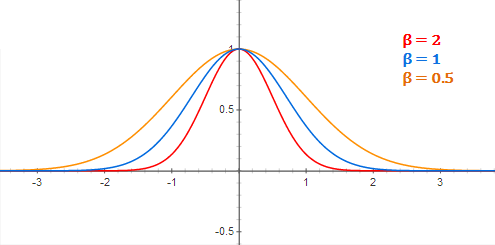
Linear Basis Function
- \(\mu\) = pivot
- \(\sigma^2\) = bandwidth
- Higher, smoother
- Lower, sharper
LDA
Linear Discriminant Analysis, using Fisher Linear Discriminant
Maximizes separation using multiple classes, by seeking a projection that best discriminates the data
It is also used a pre-processing step for ML application
Goals
- Find directions along which the classes are best-separated (ie, increase discriminatory information)
- Maximize inter-class distance
- Minimize intra-class distance
- It takes into consideration the scatter(variance) within-classes and between-classes
Steps
- Find within-class Scatter/Covariance matrix
\(S_w = S_1 + S_2\)
- \(S_1 \to\) Covariance matrix for class 1
- \(S_2 \to\) Covariance matrix for class 2
- Find between-class scatter matrix
-
Find Eigen Value
-
Find Eigen Vector
-
Generate LDA Projection Normalized Eigen Vector
-
Generate LDA score (projected value) in reduced dimensions
Eigen Value
- \(\lambda =\) Eigen Value(s)
- If we get multiple eigen values, we only take the highest eigen value
- It helps preserve more information. How??
- \(I =\) Identity Matrix
We are taking \(A=S_w^{-1} S_B\) because taking \(S_w^{-1}\) helps us maximize \(\frac{1}{x}, x \in S_w\)
- Hence \(x\) is minimized
- Thereby, within-class distance is minimized
Eigen Vector
- \(\lambda =\) Highest eigen value
- \(V =\) Eigen Vector