05 Data Exploration
Exploratory Data Analysis
Preliminary investigation of data, to understand its characteristics
Helps identify appropriate pre-processing technique and data mining algorithm
Involves
- Summary Statistics
- Visualization
Summary Statistics
Note: Statistics about the data \(\ne\) data itself
Robustness
Ability of a statistical procedure to handle a variety of non-normal distributions, including outliers
There is a trade-off between efficiency and robustness
Breakdown Point
Fraction of contaminated data in a dataset that can be tolerated by the statistical procedure
Univariate Summary Statistics
Minimal set of value(s) that captures the characteristics of large amounts of data, and show the properties of a distribution
| Meaning | Formula | Moment | Breakdown Point | Standard Error | Comment | |
|---|---|---|---|---|---|---|
| Mean/ Arithmetic Mean | Central tendency of distribution | \(\dfrac{\sum x_i}{n}\) | 1st | \(\dfrac{1}{n}\) | \(\dfrac{s}{\sqrt{n}}\) | |
| Trimmed Mean | \(k \%\) obs from top of dist are removed \(k \%\) obs from bottom of dist are removed \(\implies 2k \%\) obs are removed in total | \(\dfrac{k}{n}\) | \(\left( 1+\dfrac{2k}{n} \right)\dfrac{s}{\sqrt{n}}\) | For \(k>12.5\), better to instead use median | ||
| Winsorized Mean | \(k \%\) obs from top of dist are replaced with \((1-k)\)th percentile \(k \%\) obs from bottom of dist are replaced with \(k\)th percentile \(\implies 2k \%\) obs are replaced in total | \(\dfrac{k}{n}\) | \(\left( 1+\dfrac{2k}{n} \right)\dfrac{s}{\sqrt{n}}\) | For \(k>12.5\), better to instead use median | ||
| Weighted Mean | \(\dfrac{\sum w_i x_i}{n}\) | \(\dfrac{1}{n}\) | ||||
| Geometric Mean | \(\sqrt[{\Large n}]{\Pi x}\) | \(\dfrac{1}{n}\) | ||||
| Harmonic Mean | \(\dfrac{n}{\sum \frac{1}{x}}\) | \(\dfrac{1}{n}\) | Gives more weightage to smaller values | |||
| Median | Middle most observation 50th quantile | \(\begin{cases} x_{{n+1}/2}, & n = \text{odd} \\ \dfrac{x_{n} + x_{n+1}}{2}, & n = \text{even}\end{cases}\) | \(\dfrac{1}{2}\) | \(1.253 \dfrac{s}{\sqrt{n}}\) | Robust to outliers | |
| Mode | Most frequent observation | Unstable for small samples | ||||
| Variance | Squared average deviation of observations from mean | \(\dfrac{\sum (x_i - \mu)^2}{n}\) | 2nd Centralised | \(\dfrac{1}{n}\) | ||
| Standard Deviation | Average deviation of observations from mean | \(\sqrt{\text{Variance}}\) | \(\dfrac{1}{n}\) | |||
| Standard Error of mean | \(\dfrac{s}{\sqrt{n}}\) | |||||
| MAD Median Absolute Deviation | Median deviation of observations from mean | \(1.4826 \times \text{Med} \Big(\vert x_i - \text{Med}(x) \vert \Big)\) | \(\dfrac{1}{2}\) | |||
| Skewness | Direction of tail | \(\dfrac{\sum (x_i - \mu)^3}{n \sigma^3}\) \(\dfrac{3(\mu - \text{Md})}{\sigma}\) \(\dfrac{\mu - \text{Mo}}{\sigma}\) | 3rd Standardized | 0: Symmetric \([-0.5, 0.5]\): Approximately-Symmetric \([-1, 1]\): Moderately-skewed else: Higly-skewed | ||
| Kurtosis | Peakedness of distribution | \(\dfrac{\sum (x_i - \mu)^4}{n \sigma^4}\) | 4th standardized | |||
| Max | ||||||
| Min | ||||||
| Quantile | Divides distributions into 100 parts | Unstable for small datasets | ||||
| Quartile | Divides distributions into 4 parts | |||||
| Decile | Divides distributions into 10 parts | |||||
| Range | Range of values | Max-Min | Susceptible to outliers | |||
| IQR Interquartile Range | Q3 - Q1 | \(\dfrac{1}{4}\) | Robust to outliers | |||
| CV Coefficient of Variation | \(\dfrac{\sigma}{\mu}\) |
Standard Error of Statistic
- Standard deviation of statistic in sampling distribution
- Measure of uncertainty in the sample statistic wrt true population mean
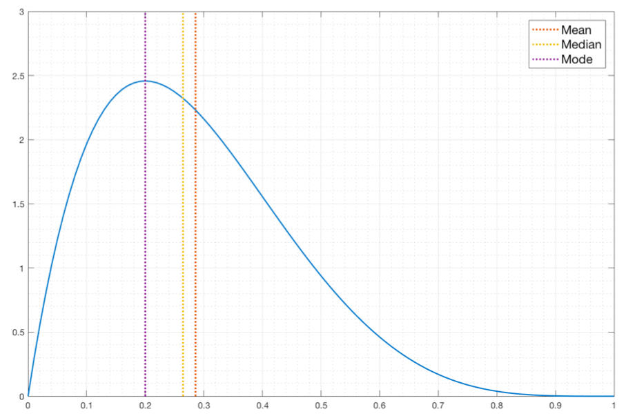
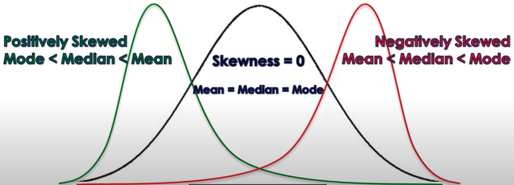
Relationship between Mean, Median, Mode
Skewness
| Skewness | Property | |
|---|---|---|
| \(> 0\) | Mode < Median < Mean | Positively Skewed |
| \(0\) | Mode = Median = Mean | |
| \(<0\) | Mean < Median < Mode | Negatively Skewed |
Moment
Multivariate Summary Statistics
| How 2 variables vary together | Covariance | \(-\infty < C < +\infty\) |
| Correlation | \(-1 \le r \le +1\) |
Covariance Matrix
It is always \(n \times n\), where \(n =\) no of attributes
| \(A_1\) | \(A_2\) | \(A_3\) | |
|---|---|---|---|
| \(A_1\) | \(\sigma^2_{A_1}\) | \(\text{Cov}(A_1, A_2)\) | \(\text{Cov}(A_1, A_3)\) |
| \(A_2\) | \(\text{Cov}(A_2, A_1)\) | \(\sigma^2_{A_2}\) | \(\text{Cov}(A_2, A_3)\) |
| \(A_3\) | \(\text{Cov}(A_3, A_1)\) | \(\text{Cov}(A_3, A_2)\) | \(\sigma^2_{A_3}\) |
The diagonal elements will be variance of the corresponding attribute
Correlation Matrix
| \(A_1\) | \(A_2\) | \(A_3\) | |
|---|---|---|---|
| \(A_1\) | \(1\) | \(r(A_1, A_2)\) | \(r(A_1, A_3)\) |
| \(A_2\) | \(r(A_2, A_1)\) | \(1\) | \(r(A_2, A_3)\) |
| \(A_3\) | \(r(A_3, A_1)\) | \(r(A_3, A_2)\) | \(1\) |
The diagonal elements will be 1
Why \((n-k)\) for sample statistics?
where \(k=\) No of estimators
- High probability that variance of sample is low, so we correct for that
- Lost degree of freedom
Standard error of mean
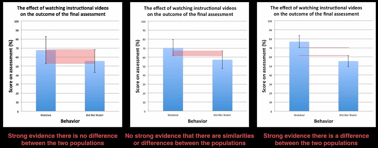
| Error bars overlap | Error bars contain both the sample means | Inference |
|---|---|---|
| ✅ | ✅ | Strong evidence that populations are not different |
| ✅ | ❌ | No strong evidence that populations are not different |
| ❌ | ❌ | Strong evidence that populations are different |