Recurrent Neural Networks
A recurrent neural network (RNN) is a NN architecture mainly used for sequences, such as speech recognition and natural language processing (NLP).

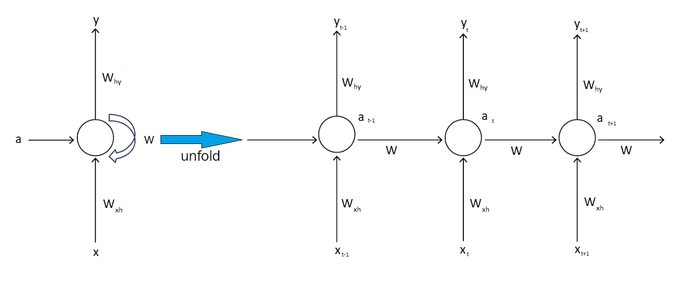
A recurrent neural network looks similar to a traditional neural network except that a memory-state is added to the neurons.
At every time step, the following are the same - function - set of parameters


A RNN cell is a neural network that is used by the RNN.
As you can see, it’s the same cell repeats over time. The weights are updated as time progresses.
IDK
We introduce a latent variable, that summarizes all the relevant information about the past


Hidden State Update
Observation Update
Advantages
- Require much less training data to reach the same level of performance as other models
- Improve faster than other methods with larger datasets
- Distributed hidden state allows storage of information about pass efficiently
- Non-linear dynamics allows them to update their hidden state in complicated ways
- With enough neurons & time, RNNs can compute anything that can be done by a computer
- Good behaviors
- Can oscillate (good for motor control)
- Can settle to point attractors (good for retrieving memories)
- Can behave chaotically (bad for info processing)
Disadvantages
- High training cost
- Difficulty dealing with long-range dependencies
- Order of input samples affects the model
- Poor gradient flow
- vanishing gradients: largest eigenvalue < 1
- Can control using gradient clipping
- exploding gradients: largest eigenvalue > 1
- Can control through additive interactions by using GRU/LSTM instead
- vanishing gradients: largest eigenvalue < 1
An Example RNN Computational Graph

Implementing RNN Cell

Tokenization/Input Encoding
Map text into sequence of IDs

Granularity
| Granularity | ID for each | Limitation |
|---|---|---|
| Character | character | Spellings not incorporated |
| Word | word | Costly for large vocabularies |
| Byte Pair | Frequent subsequence (like syllables) |
Minibatch Generation
| Partitioning | Independent samples? | No need to reset hidden state? | |
|---|---|---|---|
| Random | Pick random offest Distribute sequences @ random over mini batches | ✅ | ❌ |
| Sequential | Pick random offeset Distribute sequences in sequence over mini batches | ❌ | ✅ (we can keep hidden state across mini batches) |
Sequential sampling is much more accurate than random, since state is carried through
Hidden State Mechanics
- Input vector sequence \(x_1, \dots, x_t\)
- Hidden states \(h_1, \dots, x_t\), where \(h_t = f(h_{t-1}, x_t)\)
- Output vector sequence \(o_1, \dots, o_t\), where \(o_t = g(h_t)\)
Often outputs of current state are used as input for next hidden state (and thus output)
Output Decoding

Gradients
Long chain of dependencies for back-propagation
Need to keep a lot of intermediate values in memory
Gradients can have problems
Accuracy
Accuracy is usually measured in terms of log-likelihood. However, this makes outputs of different length incomparable (bad model on short output has higher likelihood than excellent model on very long output).
Hence, we normalize log-likelihood to sequence length
Perplexity is effectively number of possible choices on average
Truncated BPTT
Back-Propagation Through Time
| Truncation Style | |
|---|---|
| None | Costly Divergent |
| Fixed-Intervals | Standard Approach Approximation Works well |
| Variable Length | Exit after reweighing Doesn’t work better in practice |
| Random Variable |  |

Multi-Layer RNN
