Time Series Processes¶

Time Series¶

Observation of random variable ordered by time

Time series variable can be

Time series at level (absolute value)
Difference series (relative value)
- First order difference $\Delta y_t = y_t - y_{t-1}$
- Called as ‘returns’ in finance
- Second order difference $(\Delta y_t)_2 = \Delta y_t - \Delta y_{t-1}$

Univariate Time Series¶

Basic model only using a variable’s own properties like lagged values, trend, seasonality, etc

Why do we use different techniques for time series?¶

This is due to

behavioral effect
history/memory effect
- Medical industry always looks at the records of your medical history
Inertia of change
Limited data

Components of Time Series Processes¶

	Characteristic	Frequency
Auto-Correlation
Level	Average value of series
Trend	Gradual	Low
Seasonality		Daily, Weekly, Monthly
Cycles		> 1 year	Economy cycle
Holidays			Eid, Christmas
Drift	Exogeneous
Structural Break
Shocks
Noise	Random	High

Auto-correlation¶

High possibility of auto-correlation

Sometimes just auto-correlation is enough to learn the values of a value

\[ y_t = \beta_0 + \beta_1 y_{t-1} + e_t \]

If we take $j$ lags,

\[ y_t = \beta_0 + \sum_{i=1}^j \beta_i y_{t-i} + e_t \]

Generally, $i>j \implies \beta_i < \beta_j$

Impact of earlier lags is lower than impact of recent lags

Shock¶

‘Shock’ is an abrupt/unexpected deviation(inc/dec) of the value of a variable from its expected value

This incorporates influence of previous disturbance

They cause a structural change in our model equation. Hence, we need to incorporate their effect.

\[ \text{Shock}_t = y_t - E(y_t) \]

Basically, shock is basically $u_t$ but it is fancily called as a shock, because they are large $u$

Can be

	Temporary	Permanent
Duration	Short-term	Long-Term
		Causes structural change
Examples	Change in financial activity due to Covid	Change in financial activity due to 2008 Financial Crisis
	Heart rate change due to minor stroke Heart rate change due to playing	Heart rate change due to major stroke Heart rate change due to big injury
	Goals scored change due to small fever	Goals scored change due to big injury

Model becomes

\[ y_t = \beta_0 + \beta_1 y_{t-1} + \beta_2 u_{t-1} \]

Structural Breaks¶

Permanent change in the variable causes permanent change in relationship

We can either use

different models before and after structural break
binary ‘structural dummy variable’ to capture this effect

For eg, long-term injury

\[ y_t = \beta_0 + \beta_1 y_{t-1} + \beta_2 B_t \]

Trend¶

Tendency of time series to change at a certain expected rate.

Trend can be

deterministic/systematic (measurable)
random/stochastic (not measurable $\implies$ cannot be incorporated)

For eg: as age increases, humans have a trend of

growing at a certain till the age of 20 or so
reducing heart rate

Model becomes

\[ y_t = \beta_0 + \beta_1 y_{t-1} + \beta_2 t \]

Seasonality/Periodicity¶

\[ y_t = \beta_0 + \beta_1 y_{t-1} + \beta_2 \textcolor{hotpink}{S} + \beta_3 \textcolor{hotpink}{t S} \]

Tendency of a variable to change in a certain manner at regular intervals.

For eg

demand for woolen clothes is high every winter
demand for ice cream is high every summer

Finance industry has ‘anomalies’

Two ways to encode

Type	Advantage	Disadvantage	Example	$S$
Binary	Simple	Unrealistic	Dummy	$\{0, 1\}$
Continuous	Realistic	Complex	Cyclic Linear Basis	$\exp{\left[\frac{- 1}{2 \alpha^2} (x_i - \text{pivot})^2\right]}$ - Pivot is the center of the curve	Preferred, as more control over amplitude and bandwidth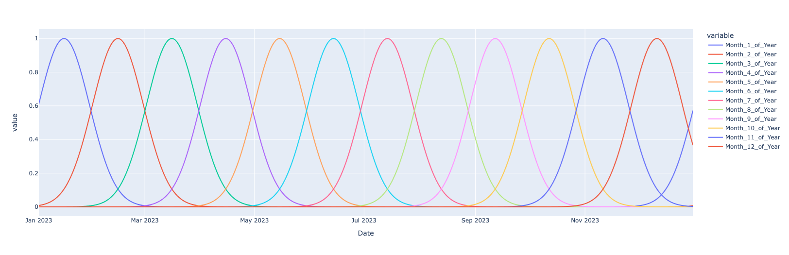
			Fourier series	$\alpha \cos \left(\frac{2 \pi}{\nu} + \phi \right) + \beta \sin \left( \frac{2 \pi}{\nu} + \phi\right)$, where $\nu =$ Frequency of seasonality, and $\phi$ is the offset - Quarterly = 4 - Monthly = 12

Volatility¶

Annualized standard deviation of change of a random variable

Measure of variation of a variable from its expected value

If the variance is heteroskedastic (changes over time), the variable is volatile

\[ \begin{aligned} \sigma^2_{y_t} &= E \Big [\Big(y_t - E(u_t) \Big)^2 \Big] \\ &= E \Big [\Big(y_t - \textcolor{hotpink}{0} \Big)^2 \Big] \\ &= E [y_t^2 ] \\ &= y_t^2 \\ \end{aligned} \]

\[ y_t = \beta_0 + \beta_1 y_{t-1} + \beta_2 \sigma^2_{t-1} \]

Lag Terms¶

\[ \begin{aligned} \text{Let's say} \to y_t &= f(y_{t-2}) \\ y_t &= f(y_{t-1}) \\ y_{t-1} &= f(y_{t-2}) \end{aligned} \]

\[ y_t = \rho_1 y_{t-1} + \rho_2 y_{t-2} + u_t \]

Here, $\rho_1$ and $\rho_2$ are partial-autocorrelation coefficient of $y_{t-1}$ and $y_{t-2}$ on $y_t$

\[ y_t = \rho_1 y_{t-2} + u_t \]

Here, $\rho_1$ is total autocorrelation coefficient of $y_{t-2}$ on $y_t$

We choose the number of lags by trial-and-error and checking which coefficients are significant ($\ne 0$)

Stochastic Data-Generating Processes¶

Stochastic process is a sequence of random observations indexed by time

Markov Chain¶

Stochastic process where effect of past on future is summarized only by current state $$ P(y_{t+1} = a \vert x_0, x_1, \dots x_t) = P(x_{t+1} = a \vert x_t) $$ If possible values of $x_i$ is a finite set, MC can be represented as a transition probability matrix

Martingale¶

Stochastic processes which are a “fair” game $$ E[y_{t+1} \vert y_t] = y_t $$ Follow optimal stopping theorem

Subordinated¶

Stationarity¶

Type	Meaning
Stationary	Constant mean: $E(y_t) = \mu$ Constant variance: $\text{Var}(y_t) = \sigma^2$
Covariance Stationary	Constant mean: $E(y_t) = \mu$ Constant variance: $\text{Var}(y_t) = \sigma^2$ Constant auto-covariance: $\text{Cov}(y_{t+h}, y_t) = \gamma(\tau)$
Non-Stationary	Will have either one/both of the following - Mean at each time period is different across all time periods - Mean of distribution of possible outcomes corresponding to each time period is different - Variance at each time period is different across all time periods - Variance of distribution of possible outcomes corresponding to each time period is different We need to transform this somehow, as OLS and GMM cannot be used for non-stationary processes, because the properties of OLS are violated - heteroskedastic variance of error term

Types of Stochastic Processes¶

Consider $u_t = N(0, \sigma^2)$

Process	Characteristics	$y_t$	Comments	Mean	Variance	Memory	Example
White Noise	Stationary	$u_t$	PAC & TAC for each lag = 0	0	$\sigma^2$	None	If a financial series is a white noise series, then we say that the ‘market is efficient’
Ornstein Uhlenbeck Process/ Vasicek Model	Stationary Markov chain	$\beta_1 y_{t-1} + u_t; \ 0 < \vert \beta_1 \vert < 1$	Series has Mean-reverting Earlier past is less important compared to recent past. Less susceptible to permanent shock Series oscilates	0/non-zero	$\sigma^2$	Short	GDP growth Interest rate spreads Real exchange rates Valuation ratios (divides-price, earnings-price)
Covariance Stationary		$y_t = V_t + S_t$ (Wold Representation Theorem) $V_t$ is a linear combination of past values of $V_t$ with constant coefficients $S_t = \sum \psi_i u_{t-i}$ is an infinite moving-average process of error terms, where $\psi_0=1, \sum \psi_i^2 < \infty$; $\eta_t$ is linearly-unpredictable white noise and $u_t$ is uncorrelated with $V_t$
Simple Random Walk	Non-Stationary Markov chain Martingale	$\begin{aligned} &= y_{t-1} + u_t \\ &= y_0 + \sum_{i=0}^t u_i \end{aligned}$	PAC & TAC for each lag = 0 $y_{t+h} - y_t$ has the same dist as $y_h$	$y_0$	$t \sigma^2$	Long
Explosive Process	Non-Stationary	$\beta_1 y_{t-1} + u_t; \ \vert \beta_1 \vert > 1$
Random Walk w/ drift	Non-Stationary	$\begin{aligned} &= \beta_0 + y_{t-1} + u_t \\ &= t\beta_0 + y_0 + \sum_{i=0}^t u_i \end{aligned}$		$t \beta_0 + y_0$	$t \sigma^2$	Long
Random Walk w/ drift and deterministic trend	Non-Stationary	$\begin{aligned} &= \beta_0 + \beta_1 t + y_{t-1} + u_t \\ &= y_0 + t \beta_0 + \beta_1 \sum_{i=1}^t i + \sum_{i=1}^t u_t \end{aligned}$		$t \beta_0 + \beta_1 \sum_{i=1}^t i + y_0$	$t \sigma^2$	Long
Random Walk w/ drift and non-deterministic trend	Non-Stationary	Same as above, but $\beta_1$ is non-deterministic

Impulse Response Function of covariance stationary process $y_t$ is $$ \begin{aligned} \text{IR}(j) &= \dfrac{\partial y_t}{\partial \eta_{t-j}} \ &= \psi_j \ \implies \sum \text{IR}(j) &= \phi(L), \text{with L=}1 \ &\text{ (L is lag operator)} \end{aligned} $$

Differentiation¶

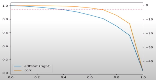
When converting a non-stationary series $y_t$ into a stationary series $y'_t$, we want

Obtain stationarity: ADF Stat at 95% CL as $-2.8623$
Retain memory: Similarity to original series; High correlation b/w original series and differentiated series

\[ y'_t = y_t - d y_{t-1} \\ d \in [0, 1] \\ d_\text{usual} \in [0.3, 0.5] \]

$d$	Stationarity	Memory
0	❌	✅
$(0, 1)$ (Fractional differentiation)	✅	✅
1	✅	❌

Integrated/DS Process¶

Difference Stationary Process

A non-stationary series is said to be integrated of order $k$, if mean and variance of $k^\text{th}$-difference are time-invariant

If the first-difference is non-stationary, we take second-difference, and so on

Pure random walk is DS¶

\[ \begin{aligned} y_t &= y_{t-1} + u_t \\ \implies \Delta y_t &= \Delta y_{t-1} + u_t \quad \text{(White Noise Process = Stationary)} \end{aligned} \]

Random walk w/ drift is DS¶

\[ \begin{aligned} y_t &= \beta_0 + y_{t-1} + u_t \\ \implies \Delta y_t &= \beta_0 + \Delta y_{t-1} + u_t \quad \text{(Stationary)} \end{aligned} \]

TS Process¶

Trend Stationary Process

A non-stationary series is said to be …, if mean and variance of de-trended series are time-invariant

Assume a process is given by

\[ y_t = \beta_0 + \beta_1 t + y_{t-1} + u_t \]

where trend is deterministic/stochastic

Then

Time-varying mean
Constant variance ???

We perform de-trending $\implies$ subtract $(\beta_0 + \beta_1 t)$ from $y_t$

\[ (y_t - \beta_0 - \beta_1 t) = y_{t-1} + u_t \]

If

$\beta_2 = 0$, the de-trended series is white noise process
$\beta_2 \ne 0$, the de-trended series is a stationary process

Note Let’s say $y_t = f(x_t)$

If both $x_t$ and $y_t$ have equal trends, then no need to de-trend, as both the trends will cancel each other

Unit Root Test for Process Identification¶

\[ y_t = \textcolor{hotpink}{\beta_1} y_{t-1} + u_t \]

$\textcolor{hotpink}{\beta_1}$	$\gamma$	Process
$0$		White Noise
$(0, 1)$		Stationary
$[1, \infty)$		Non-Stationary

Augmented Dicky-Fuller Test¶

$H_0: \beta_1=1$
$H_0: \beta_1 \ne 1$

Alternatively, subtract $y_{t-1}$ on both sides of main equation

\[ \begin{aligned} y_t - y_{t-1} &= \beta_1 y_{t-1} - y_{t-1} + u_t \\ y_t - y_{t-1} &= (\beta_1-1) y_{t-1} + u_t \\ \Delta y_t &= \gamma y_{t-1} + u_t & (\gamma = \beta_1 - 1) \end{aligned} \]

$H_0: \gamma=1$ (Non-Stationary)
$H_1: \gamma \ne 1$ (Stationary)

If p value $\le 0.05$

we reject null hypothesis and accept alternate hypothesis
Hence, process is stationary

We test the hypothesis using Dicky-Fuller distribution, to generate the critical region

Model	Hypotheses $H_0$	Test Statistic
$\Delta y_t =$

Long memory series¶

Earlier past is as important as recent past

Q Statistic¶

Test statistic like $z$ and $t$ distribution, which is used to test ‘joint hypothesis’

Inertia of Time Series Variable¶

Persistance of value due to Autocorrelation

Today’s exchange rate is basically yesterday’s exchange rate, plus-minus something

Last Updated: 2024-05-12 ; Contributors: AhmedThahir

\(\textcolor{hotpink}{\beta_1}\)	\(\gamma\)	Process
\(0\)		White Noise
\((0, 1)\)		Stationary
\([1, \infty)\)		Non-Stationary

Type	Meaning
Stationary	Constant mean: \(E(y_t) = \mu\) Constant variance: \(\text{Var}(y_t) = \sigma^2\)
Covariance Stationary	Constant mean: \(E(y_t) = \mu\) Constant variance: \(\text{Var}(y_t) = \sigma^2\) Constant auto-covariance: \(\text{Cov}(y_{t+h}, y_t) = \gamma(\tau)\)
Non-Stationary	Will have either one/both of the following - Mean at each time period is different across all time periods - Mean of distribution of possible outcomes corresponding to each time period is different - Variance at each time period is different across all time periods - Variance of distribution of possible outcomes corresponding to each time period is different We need to transform this somehow, as OLS and GMM cannot be used for non-stationary processes, because the properties of OLS are violated - heteroskedastic variance of error term

Process	Characteristics	\(y_t\)	Comments	Mean	Variance	Memory	Example
White Noise	Stationary	\(u_t\)	PAC & TAC for each lag = 0	0	\(\sigma^2\)	None	If a financial series is a white noise series, then we say that the ‘market is efficient’
Ornstein Uhlenbeck Process/ Vasicek Model	Stationary Markov chain	\(\beta_1 y_{t-1} + u_t; \ 0 < \vert \beta_1 \vert < 1\)	Series has Mean-reverting Earlier past is less important compared to recent past. Less susceptible to permanent shock Series oscilates	0/non-zero	\(\sigma^2\)	Short	GDP growth Interest rate spreads Real exchange rates Valuation ratios (divides-price, earnings-price)
Covariance Stationary		\(y_t = V_t + S_t\) (Wold Representation Theorem) \(V_t\) is a linear combination of past values of \(V_t\) with constant coefficients \(S_t = \sum \psi_i u_{t-i}\) is an infinite moving-average process of error terms, where \(\psi_0=1, \sum \psi_i^2 < \infty\); \(\eta_t\) is linearly-unpredictable white noise and \(u_t\) is uncorrelated with \(V_t\)
Simple Random Walk	Non-Stationary Markov chain Martingale	\(\begin{aligned} &= y_{t-1} + u_t \\ &= y_0 + \sum_{i=0}^t u_i \end{aligned}\)	PAC & TAC for each lag = 0 \(y_{t+h} - y_t\) has the same dist as \(y_h\)	\(y_0\)	\(t \sigma^2\)	Long
Explosive Process	Non-Stationary	\(\beta_1 y_{t-1} + u_t; \ \vert \beta_1 \vert > 1\)
Random Walk w/ drift	Non-Stationary	\(\begin{aligned} &= \beta_0 + y_{t-1} + u_t \\ &= t\beta_0 + y_0 + \sum_{i=0}^t u_i \end{aligned}\)		\(t \beta_0 + y_0\)	\(t \sigma^2\)	Long
Random Walk w/ drift and deterministic trend	Non-Stationary	\(\begin{aligned} &= \beta_0 + \beta_1 t + y_{t-1} + u_t \\ &= y_0 + t \beta_0 + \beta_1 \sum_{i=1}^t i + \sum_{i=1}^t u_t \end{aligned}\)		\(t \beta_0 + \beta_1 \sum_{i=1}^t i + y_0\)	\(t \sigma^2\)	Long
Random Walk w/ drift and non-deterministic trend	Non-Stationary	Same as above, but \(\beta_1\) is non-deterministic