07 Elasticity
Elasticity
Partial derivatives are not a good way for comparing sensitivity, as unit of measurement is different and hence cannot be used
- for different commodities, or
- in different locations
Elasticity is better
- unit-free
- different goods
- different locations
Price Elasticity of Demand
Proportional change in demand of commodity wrt proportional change in price of that commodity
measure/responsives of the demand of a commodity to a given change in price, in terms of %
\(e\) is generally negative (demand is generally negatively-related) but for giffen goods, \(e\) is positive
if price of commodity changes by some \(k \%\), demand for it changes by \(k \times e \%\)
Types
Note that the following shows the magnitude only
| \(\vert e_x^p \vert\) | Demand |
|---|---|
| 0 | perfectly inelastic (demand curve vertical - parallel to price axis) |
| \(0 < \vert e \vert < 1\) | inelastic (low sensitivity) |
| 1 | unitary elastic |
| \(1 < \vert e \vert < \infty\) | elastic |
| \(\infty\) | perfectly elastic (demand curve horizontal - parallel to demand axis) happens in perfectly-competitive market |

Cases
Consider profit functions \(\pi_1 = f_1(R, \dots), \pi_2 = f_2(R, \dots),\) where
- \(\pi =\) profit of company
- R = revenue (incorporates pricing of both companies)
Now - if \(\frac{\delta \pi_2}{\delta \pi_1} = 0,\) perfectly competitive market the profits of one company is independent of the profits of another company - eg: agricultural farmers - else imperfect market - eg: aviation industry
Cross Price Elasticity of Demand
Proportional change in demand of commodity wrt proportional change in price of another commodity
proportional change may be % change
if price of another commodity changes by some \(k \%\), demand of our main commodity changes by \(k \times e \%\)
Sign
- -ve for complimentary goods
- 0 for insensitive
- +ve for substitute goods
Magnitude
shows the degree of complimentarity/substitutability
Determinants of Elasticity of Demand
i’m using \(|e|\) to highlight only the magnitude
Availability of substitute
- more substitutes, more elastic
- coke, pepsi
- rice, wheat
- no substitutes, inelastic
- petrol
- water
Type of commodity
- Luxury goods - elastic \(|e| \to \infty\)
- Necessities - inelastic \(|e| \to 0\)
No of purposes/uses for commodity
more uses, more elastic
- eg: milk, steel
- if price increases, you will stop using for less important stuff
fewer purposes, less elastic
- eg: petrol
- even if prices change, nothing really changes, you can only use petrol for car
Proportion of income spent on commodity
more prop of income required, price elastic
- what you buy very frequently
- milk, petrol
less prop of income required, price inelastic
- what you buy less frequently
- eg: flight tickets, junk food, noodles for me
Time Period
- In the shortrun, demand is inelastic
- In the longrun, demand is elastic
There is more time for consumers to reconsider their decision, to see if it is actually necessary to do so
Addictiveness
- More addictive product is inelastic
- less addictive product is elastic
Income Elasticity
Total Revenue
basically finding the relationship bw TR and demand
Graph
- y = price
- x = Total Revenue
Changes in total revenue depends on
- quantity demand
- elasticity of demand
The change is based on which factor is of greater magnitude
Inelastic
For necessities, when price increases, total revenue increases
reduction in price is pointless, and increase in price is good for profits
Unitary Elastic
graph is vertical line parallel to price
proportion of consumers’ income spend does not change with change in price
Elastic
For luxury goods, when price increases, total revenue decreases
discounts and offers is always a good policy, cuz the inc in profit due to inc in demand > dec in profits due to dec in price
TR using Graph
normal price-demand graph
TR = quantity x price = area under graph
with change in price
- For inelastic demand, the area of graph has minimal change
- For elastic demand, the area of graph has significant change
Various Points of Graph
draw geogebra graph
- At greater price, demand is elastic
- At center point, demand is unitary elastic
- At lower price, demand is inelastic
Revenue is greatest at center point
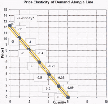
This is due to Point Elasticity
eg: if price of car goes from 100k to 50k, so many more people will buy but if price of car goes from 10k to 5k, not that many more people will buy
Income Elasticity
Proportional change in demand of commodity wrt proportional change in income of consumers
For inferior goods, \(- \infty < e < 0\)
For normal goods, \(0 < e < \infty\)
- For necessities \(e \to 0\)
- income inelastic
- For luxury goods, \(e \to \infty\)
Relation bw Income Elasticity and Price Elasticity
\(e^p \propto e^m\) High Income Elasticity \(\implies\) High Price Elasticity
This is because of
-
substitution effect
- when price decreases, you start buying more
- when price increases, you just don’t buy this product and start buying alternatives
-
income effect
the real income gets changed
- when price decreases, you feel richer, cuz you can now buy more
- when price increases, you feel poorer, cuz you can now buy less
Midpoint Formula for % change
Good as it gives the same answer regardless of direction of change
helpful when we don’t know what the initial value, ie we don’t know what \(\frac p x\) is
let \(v\) be the value
Elasticity of Supply
Proportional change in the supply of a commodity wrt proportional change of its price
Always \(0 < e < \infty\)
perfectly inelastic
-
\(e \propto T\)
- sellers have small time to revise their decisions
- Real Estate in short run
-
\(e \propto \frac 1 G\)
- or where gestation period is long(time taken to convert raw materials into final good)
- eg: agrigultural, large machinery
Perfectly elastic
perfectly competitive market

Factors of Elasticity of Supply
Nature of Commodity
supply is elastic if it is possible to change the amount produced
- it is not possible for real estate
- it is possible for books, cars, manufactured goods
Time
supply is more elastic if suppliers have time to respond
supply is more elastic in long run, as there is time to find alternatives
- oil was nearly inelastic before cuz there were no other alternatives
- but now, suppliers have to make decision on production quantity based on how much they think the consumers will buy, as there are other alternatives
Interesting question on farmer
based on total revenue
in slides
- the relation for eggs is lagged; the supplier wouldn’t know the future price
- but for oil, they can do it instantly
but the breaking eggs and reducing oil production only works in the short run, cuz consumers will find other alternatives
for medicines, technological change is disliked by pharmaceutical companies
but for luxury goods and computer manufacturing it is opposite, cuz demand for computers is elastic; so decrease in price would increase the total revenue
Applications
OPEC
(above)
Drugs
2 options to address
- Interdiction: cracking down on suppliers and restrict the supply for drugs
- Education: reduce the demand for drugs
Keeping in mind that drugs are price-inelastic, education is more effective cuz
| Interdiction | Education | |
|---|---|---|
| supply | dec | same |
| demand | same | dec |
| price | inc | dec |
| surviving cartels | richer | poorer |
| addicts | poorer | better off |
| crime | inc | dec |
Immigration
the increase in price for luxury housing will be greater than that for cars
| supply | demand | |
|---|---|---|
| luxury housing | inelastic | elastic |
| cars | elastic | elastic |
Point Elasticity
This wasn’t taught in class, but I came across during Study Project research.
Point elasticity is the elasticity at a point, duh.
We know that elasticity is \(e_x^p = \dfrac{\Delta x}{\Delta p} \dfrac{p}{{x}}\). But for a single point, we do not have \(\Delta x\) and \(\Delta p\). So what we do is we take the slope of the graph instead.
So the point elasticity of any point is